F.A.Q.
For most applications the "bins" will be of interest as these are defined with respect to all the sequences. So you can actually ignore the clusters as these represent intermediate results which are presented for completeness reasons.
The BusyBee Web server uses BusyBee (a command-line binning solution) to perform the unsupervised binning, which is central to the entire workflow. As metagenomic datasets grow larger and larger, it was important to implement an efficient way of defining sequence groups (clusters/bins) and to assign sequences to individual groups.
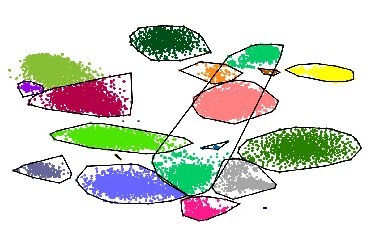
Based on our experience from the development of VizBin, BusyBee first defines a set of clusters on a subset of all the sequences. This is where the "border points threshold" and the "cluster points threshold" come ino play. The higher these thresholds are set, the fewer sequences will be used for cluster definition. Of course, clustering too few or too may sequences is undesirable. Hence, we suggest to set these values depending on the total amount of sequences and they are set to relatively small values by default. This is important to properly process highly fragmented assemblies.
After the individual clusters are defined from the border points and cluster points, this information is used to train a classifier. The classifier, in turn, is used to assign cluster labels to all the sequences, i.e., regardless whether they are border points, cluster points, or shorter points. The sequence groups that result from the classification step are what we call bins. This combination of unsupervised (clustering) and supervised (classification) machine learning, provides a great speedup for larger datasets, while preserving high degrees of sensitivity and precision.
We suggest to skip the "functional annotation" option when starting with the analysis of a new metagenomic da taset. We think that it is important to get some impression about the "complexity" of the data first. This can be easily and quickly achieved using the BusyBee Web server.
Depending on the sequence length distribution, i.e., whether your assembly is highly fragmented or consists of few but long contigs, you can increase the "border points threshold" and "cluster points threshold", and/or increase the compression value. Increasing any of these value will lead to a reduction in the number of sequences that will be visualized and , thus, will lead to quicker turnaround times. For example, choosing a compression value of "1" will reduce the visualized data to about 50%, and a compression value of "2" will reduce it to about 33%. As you can see, a small compression value can already markedly reduce the number of points to be visualized and thus the runtime.
This way, you can quickly get an overview of the "complexity" of your data, e.g., the number of distinct bins to expect, or whether there is a great difference in the assembly quality of individual genomes/bins. Once you have this overview, choosing the right parameter values should be more apparent, e.g., you might want to increase or decrease the minimum number of points to define a cluster depending on whether you observe many "mini"-clusters of low completeness or many clusters that are separate according to your visual inspection but have been joined into a common cluster by the automated clustering, respectively. It could very well be that the resulting cluster structures are well defined. You could then start a more time-consuming analysis by enabling the "functional annotation" or you could simply use the resulting bins for your downstream, detailed analyses, e.g., bin-level metabolic reconstructions or phylogenetic studies.
Defining what a "perfect" bin represents is hard. Should it be complete but a certain degree of contamination is acceptable? What would then be an acceptable degree of contamination? How about "mini"-clusters? We do not want to give a single answer here as we think this highly depends on your question at hand. However, the BusyBee Web server provides you with several complementary sources of information to answer this question for yourself.
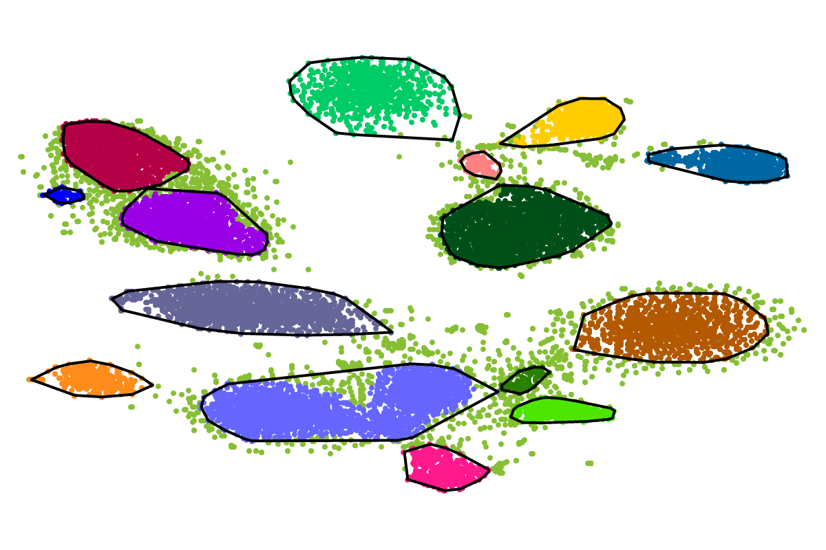
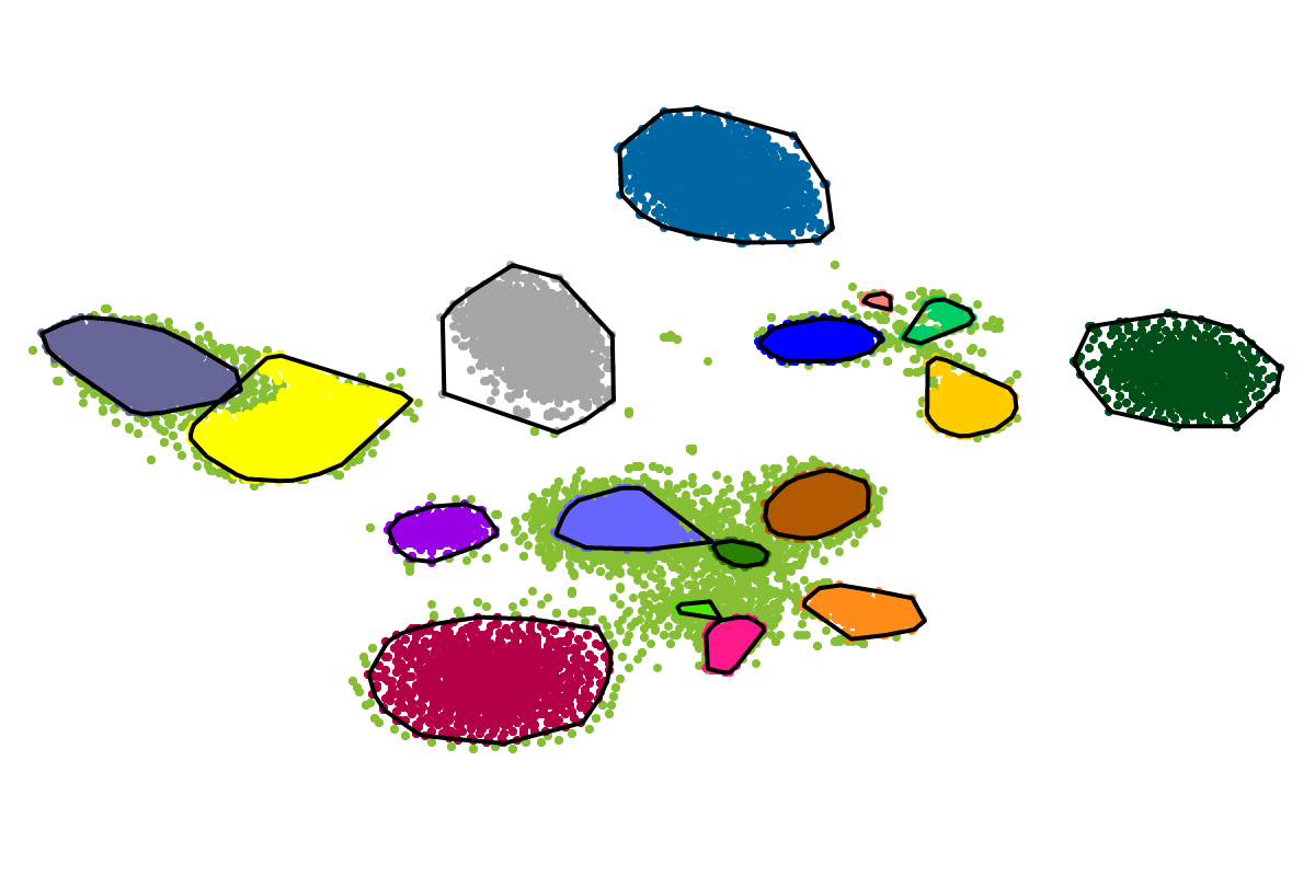
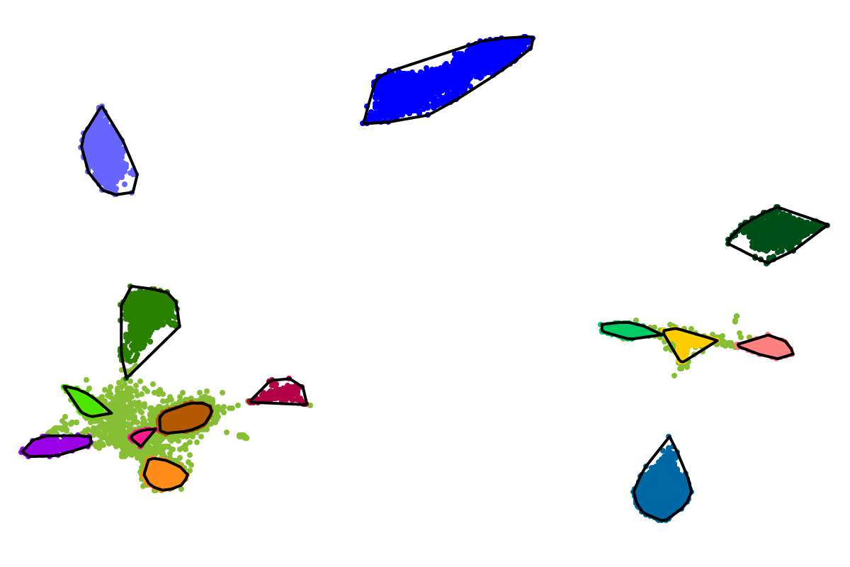
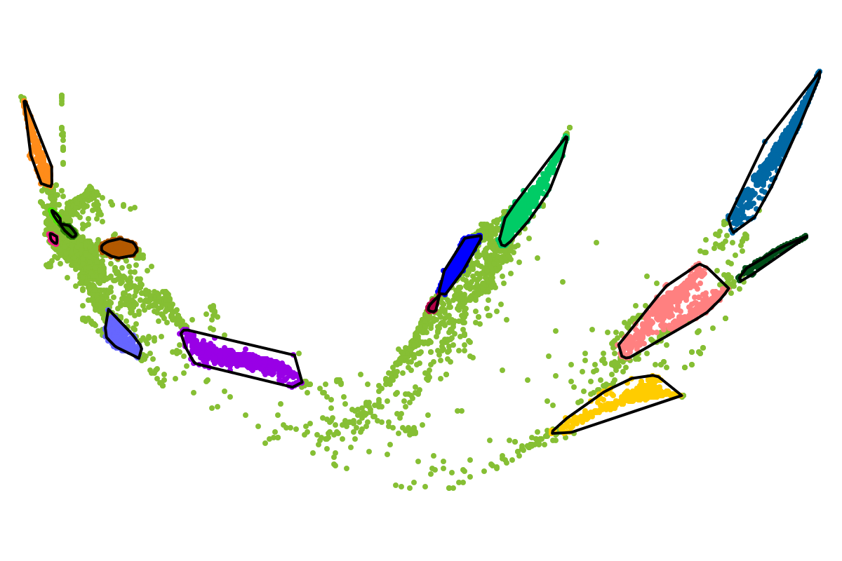
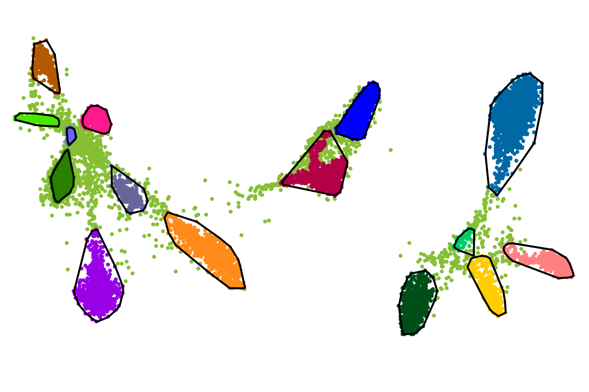
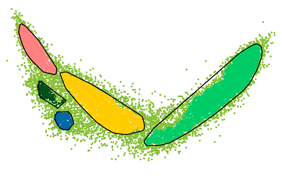
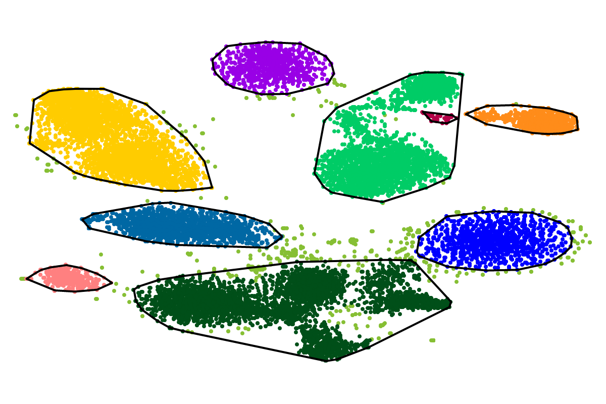
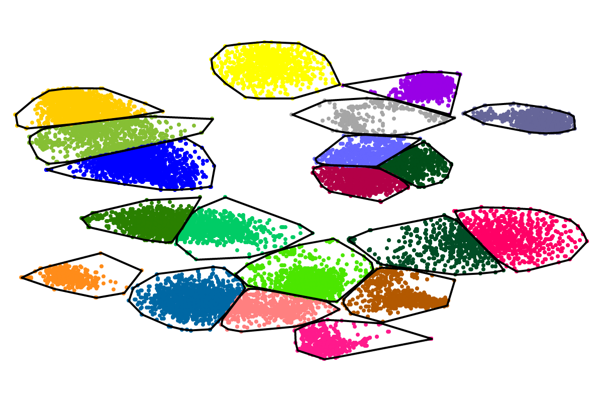
First, by simply looking at the automated clustering results in the scatterplot (2D embedding), clusters that should be separate or that should be joined ("mini"-cluster, similar to a satellite) can be readily identified. Separation of the to-be-separated clusters could be achieved by submitting the FASTA file of the respective bin to BusBee Web separately or by using VizBin to manually separate the consituent clusters. Joining clusters can either be done post-hoc, i.e., by merging the FASTA files of the "main"-cluster and the "mini"-clusters, or by submitting the same data again and, this time, choosing a larger number of minimum points
Second, the taxonomic annotation can give you an indication whether a cluster contains sequences of closely related organisms, e.g., different species of the same genus. For closely related organisms, the genomic signatures will often be very similar, thereby challenging genomic signature-based binning approaches, e.g., BusyBee Web. Here, complementary binning approaches, e.g., based on coverage, are likely to help further separate the consituent organisms. In case the taxonomic annotation was successful, i.e., the vast majority of the sequences in a bin could be assigned a taxon, inparticular at the genus- or species-level, a reference-dependent approach, e.g., BLAST, could be used to refine the bin. However, sequences specific to the organism(s) in your sample might be missed in the refinement then.
Finally, the bin quality control via single copy marker genes allows you to quantitatively asses the completeness and contamination of each bin. Generally, as low of a degree of contamination as possible is desirable. However, it could be that the contamination value of a bin is high, e.g., 200%, but at the same time, the degree of strain heterogeneity is high, e.g., 90%. This could be an indication that this bin contains two strains of the same species. Importantly, when pooling individual assemblies, e.g., from distinct timepoints, high degrees of contamination as well as strain heterogeneity are expected.
.fasta, .fa, .fsa, .fna, .ffn, .frn.
The sequences should be either assembled contigs or long reads (e.g., PacBio, ONT).
In the case of the latter, we encourage the submission of reads that do not have too many errors, i.e., "first generation" long read sequencing data.
While the sequences do not need to be "perfect", a light "polishing/error correction" is likely to contribute to more well-defined clusters and will also increase the chances of getting meaningful taxonomic and functional annotations.
Due to restraints of computational resources, we have to impose a file size limit. While this limit may change in the future, it might be that you have particularly large datasets, e.g., a few hundred-thousand sequences (contig or long reads). In this case, please contact us.
Otherwise, you might filter your sequences according to length and resubmit the reduced dataset. This will at least provide you with an initial impression what you data "looks" like and subsequent steps can be established accordingly. Moreover, BusyBee, a command line solution for offline use, can be used for larger datasets. Please contact us, should you be interested in such an option.
Alternatively, you could use VizBin which can be downloaded from here.
In order to use this option, simply provide a two-column, tab-separated text file with the first column of each line containing the sequence ID and the second column of each line containing the respective annotation. If you provided this file during job submission, BusyBee Web will use the respective annotation analogous to how it uses, e.g., the automatically generated, Kraken-based annotations, and sequences for which no custom annotation was provided will be represented as "no annotation". Accordingly, you do not need to specify annotations for each and every sequence.
For example, you could have a handful of sequences that are particularly interesting as they encode specific genes. Or, you could have annotated your sequences a priori using a custom reference genome database and you would like to overlay this information for a larger subset of the sequences. The information must be categorical and no more than 20 levels should be used. You are however free to name the individual levels. You could thus, e.g., highlight sequences according to their genomic fold-coverage ("high", "medium", "low") as a proxy for organismal abundance. Alternatively, you could use metatranscriptomic information to identify highly active organisms or a ratio of genomic and transcriptomic fold-coverage to identify, e.g., lowly abundant organisms with exceptionally high transcriptional activity.
